A Basic Vulkan Renderer
As part of the effort to get myself familiar with Vulkan, I developed a real-time renderer featuring global illumination with RTX technique 1. Aside from Dynamic Diffuse Global Illumination (DDGI) 2, ray-traced soft shadow and specular reflections with spatio-temporal denoising (SVGF 3), I've also tried out some other interesting ideas.
Visibility buffer rendering and scene management
Visibility buffer rendering 4 has gained its popularity as triangle meshes used in real-time applications are getting much finer details thanks to the rapidly increasing memory capacity and computational power of the GPU 5. More details for triangle meshes generally means fewer pixels each triangle can cover. Due to low quad utilization 6, traditional deferred shading tends to get very inefficient since there is usually a lot of computation going on in the fragment shader to fill the G-buffer.
Since there doesn't seem to be any solid reasons against it, I decided to go with visibility buffer rendering, i.e., a simple G-buffer consisting of only triangle indices and depth values. One problem needs to be addressed is how to recover the geometric data required for shading from a triangle index, including world position, normal, uv coordinates at each pixel. Moreover, We need the derivatives of uv coordinates to determine the LOD of the textures. The derivatives of the world position may be useful for e.g. constructing cotangent frame. To get the computation of partial derivatives right, I did some math and detailed the method for analytically computing partial derivatives in my last post. Another piece of information needed for shading is material data, such as textures and alpha cutoff value (for e.g. tree leaves). To simplify scene management and avoid frequently updating descriptor sets, I took a bindless approach 7. Although many mobile devices and integrated cards are not very friendly to this approach due to lack of support for Vulkan feature shaderSampledImageArrayNonUniformIndexing or VK_EXT_descriptor_indexing, or the supported limits such as maxPerStageDescriptorSampledImages are too small for typical test scenes like Sponza, GPUs that support RTX are usually very generous in this regard.
Partly due to a variety of different 3D formats, scene management can get quite complicated. Although I've dealt with .ply and .obj files while working on my master project, neither of them can really fulfill the requirement of a renderer by today's standard, at least in terms of materials that support Physically-Based Rendering (PBR). Therefore, this renderer only supports glTF format as it is royalty-free, extensible and has support for basic PBR materials among other advantages. Many other formats can be easily converted to glTF using blender. Despite the fact that glTF can store most of its data in binary form, loading glTF models that contain many textures can still be very slow because decoding common image formats (e.g. .jpg or .png) is rather computationally expensive, but directly storing the decoded image data in a cache file is not ideal either due to storage constraints. Inspired by this article, I also opted for block compression to reduce the cache file size while accelerating scene loading. To facilitate batch upload of textures to the device (GPU), I packed all the textures alongside other scene data into a single binary cache file.
Putting everything together, I came up with the following binary format for the scene cache file:
 1// metadata to determine if the cache is up-to-date
 2// punctual lights
 3// aabb lower and upper
 4vertex_offsets : uint32_t[material_type_count + 1]
 5index_offsets : uint32_t[material_type_count + 1]
 6mtl_param_emissive_idx_offsets : uint32_t[material_type_count + 1]
 7mtl_param_alpha_cutoff_offsets : uint32_t[material_type_count + 1]
 8emissive_texture_count : uint32_t // at least one black texture
 9texture_strides : uint32_t[material_type_count]
10texture_offsets : uint32_t[material_type_count + 1] // texture index offset for each mtl_type
11position_buffer
12normal_buffer
13uv_buffer
14index_buffer
15triangle_mtl_idx_buffer
16mtl_param_buffer; // array of scene_t::mtl_param_type[]
17sampler_count: uint16_t
18sampler_infos
19texture_descriptor_array
20// metadata to verify data integrity
The mesh data and material data are sorted by material types. Generally different material types need different rendering pipelines. For example, MTL_TYPE_PRIMARY corresponds to the metallic-roughness material with alphaMode set to the default value OPAQUE, while MTL_TYPE_ALPHA_CUTOFF differs only by setting alphaMode to MASK. An instance of a material type refers to a specific set of textures and material parameters.
{ vertex | index | mtl_param* | texture }_offsets are offsets of different material types in *_buffer or texture_descriptor_array. All *Factor fields in the glTF materials are either converted to 1x1 textures or multiplied into the corresponding texture.
Occlusion, metallic and roughness factors are merged into one texture as different color channels. Since emissive textures are relatively uncommon, a 1x1 black image shared by non-emissive material instances is put at the beginning of texture_descriptor_array, followed by other emissive textures. vkCmdBlitImage, C++ std::thread and parallel version of C++ standard algorithms library are used for faster generation of the cache data.
The cache file can greatly reduce the scene loading time. Here is the time it takes to load the scene Amazon Lumberyard Bistro (exterior) (glTF + textures: 898 MB; cache file: 1.05 GB) from a SSD:
| glTF 1st load | glTF 2nd load | cache 1st load | cache 2nd load | cache generation |
|---|---|---|---|---|
| 35.554 s | 21.874 s | 2.239 s | 1.334 s | 23.468 s |
The operating system (Windows) probably caches those files in RAM after the 1st load, hence the 2nd load is faster than the 1st load. The difference can be much larger for HDD. Indeed, loading the cache from my HDD for the first time can take 10 seconds, but subsequent loading only takes about 2 seconds.
During the development of scene management, I noticed something interesting about the performance of std::vector. To avoid surprising behavior, std::vector (with default allocator) forces initialization on allocation, with either default zero-initialization or user provided value. Although this is the expected behavior for many use cases, it can unnecessarily hurt performance if the requested amount of memory is huge and the entire purpose of the allocation is to fill it with fixed amount of data. std::array can be used if the size is known at compile time and reasonably small. Otherwise plain array managed by std::unique_ptr is a better option:
1const uint32_t num_f32_texels = 5592405; // texture: 2048 x 2048 x rgb, with full mipmap chain
2std::vector<glm::vec3> f32_texels(num_f32_texels, glm::vec3{}); // took 15.401600 ms
3std::vector<glm::vec3> f32_texels(num_f32_texels); // took 9.379000 ms
4std::unique_ptr<glm::vec3[]> f32_texels(new glm::vec3[num_f32_texels]); // took 0.014100 ms
Another caveat came to my notice is the propertyFlags of Vulkan memory. One common operation is to copy a chunk of data from host to device, therefore device memory is often allocated with the flag HOST_COHERENT. However, to copy data from device to host, HOST_CACHED needs to be specified instead of HOST_COHERENT. It can make a huge difference. On my laptop (RTX 2070 Mobile), it takes 61.931 ms to copy 21 MB from a HOST_VISIBLE, optionally HOST_COHERENT buffer to the host memory, but only 3.839 ms if the buffer is HOST_CACHED.
Dynamic diffuse global illumination (DDGI)
The implementation of DDGI is fairly straightforward, given the comprehensive description in the original papers 2 8 9 and some optimization techniques explained in this article. One slightly irritating thing is the additional step (VkDispatch) for simply copying the border texels after updating the irradiance textures, because synchronization is needed right before copying the border texels. One trick I've tried out is to treat the vertices of the grid for each probe as the value stored in the textures of the irradiance field. That means we need a $7 \times 7$ texture for a probe resolution of $8 \times 8$, which is slightly lower than it would haven been, but the result differs not very much. There were no obvious artifacts on the radiance probes either. Nevertheless, I decided to copy the border texels at some point. To avoid the additional kernel launch, I figured out another trick after some observation. With the help of the shader I wrote on shadertoy to visualize the octahedral mapping, the pattern of the copy operations finally became clear to me.
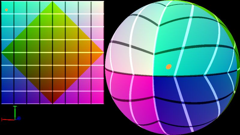
visualization of octahedral mapping
Without loss of generality, let's assume the resolution of the original probe texture is $8 \times 8$ (square with four yellow filled texels $\colorbox{#f0f010}{\textcolor{#a0a0a0}{\textsf{A}}}, \colorbox{#f0f010}{\textcolor{#a0a0a0}{\textsf{B}}}, \colorbox{#f0f010}{\textcolor{#a0a0a0}{\textsf{C}}}, \colorbox{#f0f010}{\textcolor{#a0a0a0}{\textsf{D}}}$ as its four corners in the following image), the coordinates of texel $\colorbox{#f0f010}{\textcolor{#a0a0a0}{\textsf{A}}}$ is $(0, 0)$ and $+y$ axis goes downwards, then the resolution of the padded probe texture is $10 \times 10$ with the coordinates of its top left texel being $(-1, -1)$. For texels filled with greenish or reddish color (henceforth referred to as type 1 texels), the source texel and destination texel of each copy operation need to be filled with exactly the same color. Obviously every such texel in the original probe texture is only copied once, either vertically or horizontally. It is a bit more complicated for the yellow filled texels (henceforth referred to as type 2 texels), as each of them is copied three times: vertically, horizontally and diagonally.

Some notations:
- $r$: the resolution of the original probe texture. In the image above, $r = 8$;
- $n$: maximum value of the $x-$ or $y-$coordinate of the texels in the original probe texture, clearly $n = r -1$;
- $i$: denotes $x-$ or $y-$coordinate of a texel in the original probe texture;
- Iverson bracket $[\dots]$ is used in the following definitions;
- $q_i := [ i = n]$;
- $m_i := [i = q_i \cdot n]$;
- $g_i := i + 2q_i - 1$;
- $h_i := n - i$;
- $f_i := m_i \cdot g_i + (1 - m_i) \cdot h_i$;
- $d_i := r \cdot (1 - q_i) - q_i$;
It may seem unobvious, but the type of the texel with coordinates $(x, y)$ is $m_x + m_y$. Besides, $m_i = 1$ means coordinate $i$ is mapped to $g_i$ (shifted by $\pm 1$ along the corresponding axis) and $m_i = 0$ means $i$ is mapped to $h_i$ (reflected along the corresponding axis). $f_i$ is the combined result. Type 1 texel $(x, y)$ is uniquely mapped to $(f_x, f_y)$. Type 2 texel $(x, y)$ is vertically mapped to $(g_x, h_y)$, horizontally mapped to $(h_x, g_y)$, and diagonally mapped to $(d_x, d_y)$.
With these simple functions, border texels can be copied in the same pass that updates the original probe texture, as in my implementation. Although a branch is introduced, this trick can spare us a memory barrier and another kernel launch. Since the updated probe texels still reside in registers (if no register spilling), it can help avoid some expensive global memory loads (if uncached) when copying border texels.
Spatio-temporal denoising
In this renderer, the noise comes from soft shadow and glossy reflection because of the low sampling rate (1 spp per frame for each). The (pseudo-)random numbers used for sampling are drawn from 4 blue noise textures downloaded from here. Sampling for soft shadow boils down to uniform sampling on a disk, which is fairly simple and well explained in this article. Sampling the direction of reflection for glossy materials, or equivalently sampling the normal distribution function, on the other hand, is not trivial. The implementation of the GGX VNDF Sampling 10 did the trick.
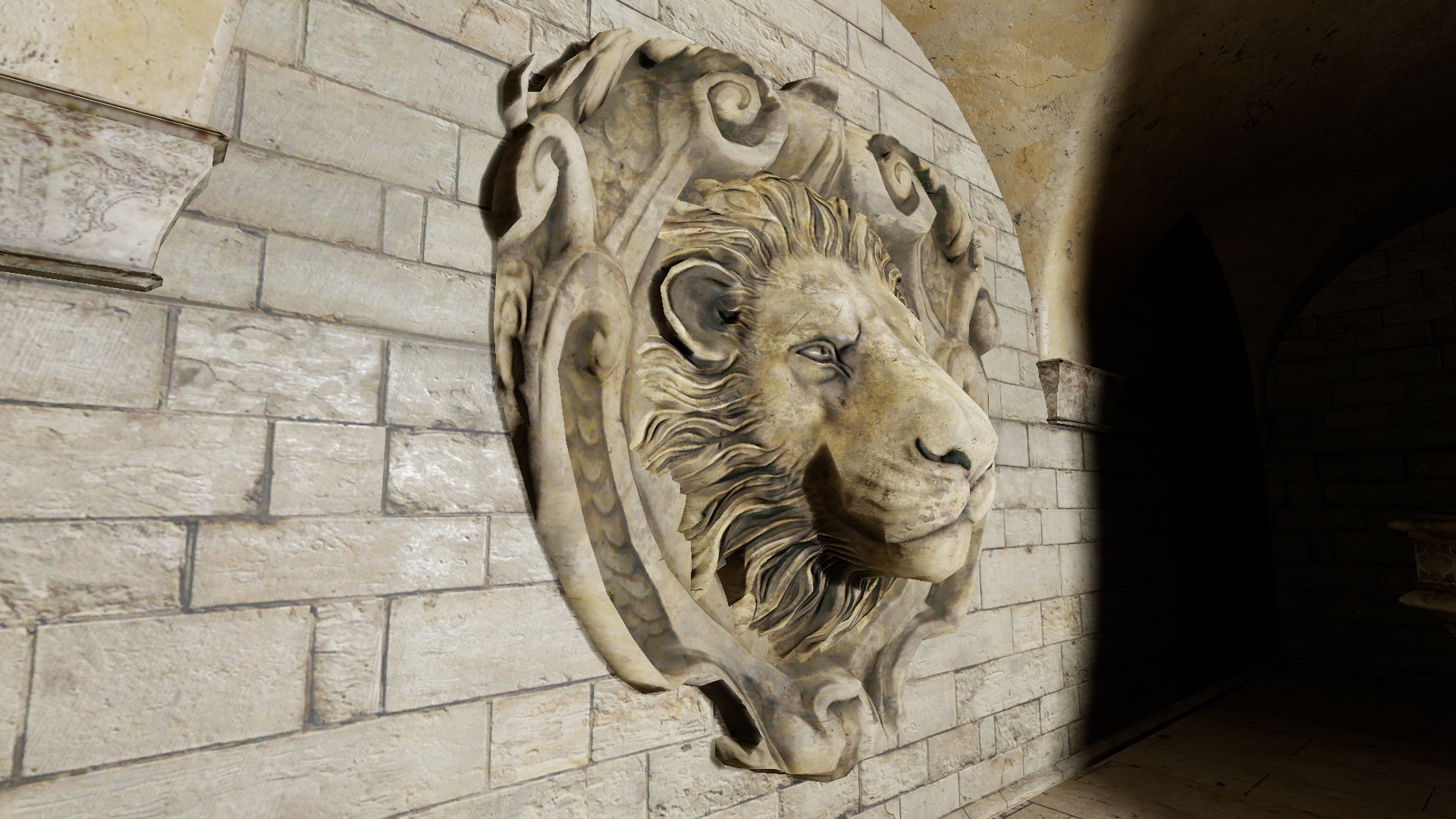
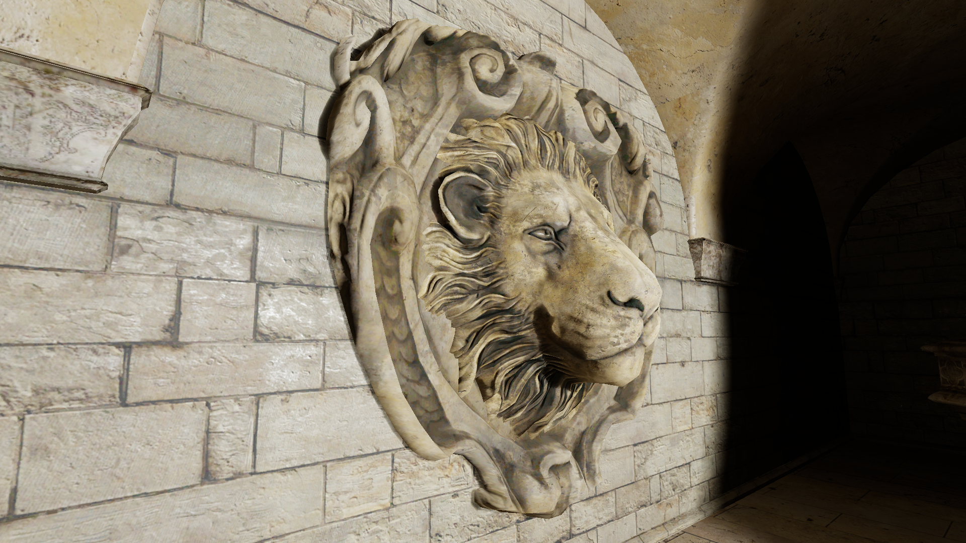
One issue with ray-traced shadow is the terminator problem caused by the fact that the smoothness of the geometry is merely approximated by the triangle meshes. If the origins of the shadow ray reside in the underlying triangles, we will inevitably get artifacts because the geometry those triangle meshes are trying to approximate is usually not flat. To work around this issue, I offset the shadow ray origins based on the vertex normals of the triangles, as explained in the article Hacking the Shadow Terminator 11. The resulting shadow is much more natural when shadow ray origin offset is applied, as shown in the following image.
For shadow denoising, I closely followed SVGF 3, which introduced a manually tunable parameter $\alpha$ to control the temporal accumulation rate. It can be seen from this video that the temporal accumulation plays an important role in the quality of the denoising. Therefore I was a bit skeptical while implementing temporal filtering technique in ReBLUR 12 for reflections because the accumulation rate is automatically adjusted. But the result turned out to be pretty satisfying. The rest of the denoising part for reflection still followed SVGF since it is already implemented in shadow denoising and I was quite confident about it.
In retrospect
Despite the renderer can run in real-time ($70+$ fps for the Sponza scene on RTX 2070 mobile), the denoising part is not optimized as it was done in haste. For example, tile-based denoising could have been used because a large portion of shadow does not need to be denoised.
DDGI is not entirely flawless either. Light/shadow leak can still happen if some probes are in suboptimal position. Besides, the hysteresis parameter that controls the pace of temporal integration cannot be set too small to avoid unstable behavior, but the lag becomes noticeable when it is very large. Next time I may try to implement something like Lumen in Unreal Engine 5.
Other interesting topics such as animation support in scene management, temporal anti-aliasing (TAA) and polygonal light should definitely be on my todo list as well.
Source code on GitLab and video on YouTube ↩︎
Zander Majercik, Jean-Philippe Guertin, Derek Nowrouzezahrai, and Morgan McGuire, Dynamic Diffuse Global Illumination with Ray-Traced Irradiance Fields, Journal of Computer Graphics Techniques (JCGT), vol. 8, no. 2, 1-30, 2019 ↩︎ ↩︎
Schied, Christoph, et al. Spatiotemporal variance-guided filtering: real-time reconstruction for path-traced global illumination. Proceedings of High Performance Graphics. 2017. 1-12. ↩︎ ↩︎
Christopher A. Burns and Warren A. Hunt, The Visibility Buffer: A Cache-Friendly Approach to Deferred Shading, Journal of Computer Graphics Techniques (JCGT), vol. 2, no. 2, 55-69, 2013 ↩︎
This article Visibility Buffer Rendering with Material Graphs provided thorough analysis and comprehensive performance test on forward shading, deferred shading and visibility buffer rendering ↩︎
See the section Bindless descriptor designs of this article ↩︎
Zander Majercik, Adam Marrs, Josef Spjut, and Morgan McGuire, Scaling Probe-Based Real-Time Dynamic Global Illumination for Production, Journal of Computer Graphics Techniques (JCGT), vol. 10, no. 2, 1-29, 2021 ↩︎
Morgan McGuire, Mike Mara, Derek Nowrouzezahrai, and David Luebke. 2017. Real-time global illumination using precomputed light field probes. In Proceedings of the 21st ACM SIGGRAPH Symposium on Interactive 3D Graphics and Games (I3D '17). Association for Computing Machinery, New York, NY, USA, Article 2, 1-11. ↩︎
Eric Heitz, Sampling the GGX Distribution of Visible Normals, Journal of Computer Graphics Techniques (JCGT), vol. 7, no. 4, 1-13, 2018 ↩︎
Hanika, J. (2021). Hacking the Shadow Terminator. In: Marrs, A., Shirley, P., Wald, I. (eds) Ray Tracing Gems II. Apress, Berkeley, CA. ↩︎
Zhdan, D. (2021). ReBLUR: A Hierarchical Recurrent Denoiser. In: Marrs, A., Shirley, P., Wald, I. (eds) Ray Tracing Gems II. Apress, Berkeley, CA. ↩︎